Let’s talk about joins
tutorials
rstats
data cleaning
data organization
An review of horizontal and vertical joins with examples from education research.
Working with data would be so much simpler if we always only had one dataset to work with. However, in the world of research, we often have multiple datasets, collected from different instruments, participants, or time periods, and our research questions typically require these data to be linked in some way. Yet, before combining data, it’s important to consider what type of join makes the most sense for our specific purposes, as well as how to correctly perform those joins. This blog post reviews the various ways we may consider combining our data.
Types of joins
In general, there are two ways to combine our data, horizontally or vertically. When linking or joining data horizontally we are matching rows by one or more variables (i.e., keys), making a wider dataset (adding columns). When joining vertically, column names are matched and datasets are stacked on top of each other, making a longer dataset (adding rows). Joins can be done in many different programs (e.g., SQL, R, Stata, SAS). Most of this post will be applicable to any language, but examples in R will be provided.
Horizontal joins
Joining data horizontally, also called merging, can be used in a variety of scenarios. A few examples include: 1. Linking data across instruments (a student survey + a student assessment) 2. Linking data across time (a student survey in the fall + a student survey in the spring) 3. Linking data across participants (a student assessment + a teacher survey) 4. Linking for de-identification purposes (a student survey with name + a student roster with study ID)
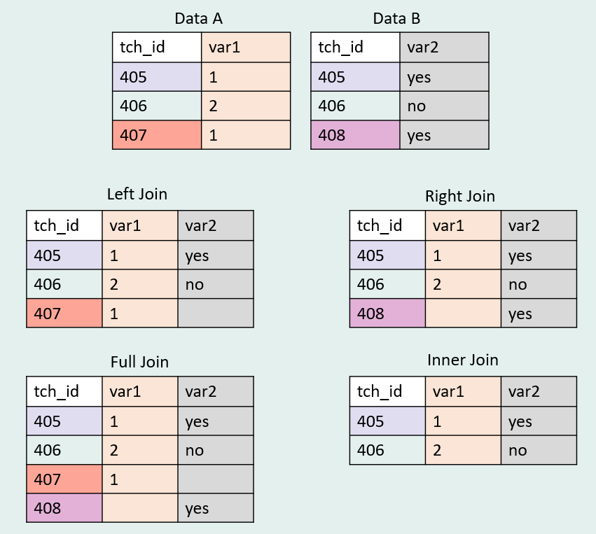
There are several different types of horizontal joins you can perform. In this post we are going to discuss mutating joins that increase the size of your dataset, as opposed to horizontal joins used for filtering data (learn more here). The four types of joins we will cover include:
- Left join
- In a left join, all cases in the dataset on the left (or our first selected dataset) are maintained. Any cases from the dataset on the left side are joined with any matching data that exists in the dataset on the right (or our second selected dataset). If additional, non-matching, cases exist in our right dataset, they will not be carried over.
- Here we typically expect that the combined dataset will have the same number of rows as our original left side dataset.
- Right join
- In a right join, all cases in the dataset on the right (or our second selected dataset) are maintained. Any cases from the dataset on the right side are joined with any matching data that exists in the dataset on the left (or our first selected dataset). If additional, non-matching, cases exist in our left dataset, they will not be carried over.
- Here we typically expect that the combined dataset will have the same number of rows as our original right side dataset.
- Full join
- In a full join, cases from both datasets are maintained. Any cases that exist in one dataset but not the other will be maintained in the final combined dataset.
- Inner join
- In an inner join, only cases that exist in both datasets will be maintained. If a case exists in one but not the other, it will not exist in the combined dataset.
There are two important rules when performing horizontal joins.
- Variable names cannot repeat.
- This means if a variable is named
genderin your student survey dataset and a variable is also namedgenderin your district records demographics dataset, those names will need to be edited (e.g., district gender can be renamed tod_gender). You can learn more about variable naming here. - This rule does not apply to your linking keys (e.g., study ID), which are often named identically across datasets.
- This means if a variable is named
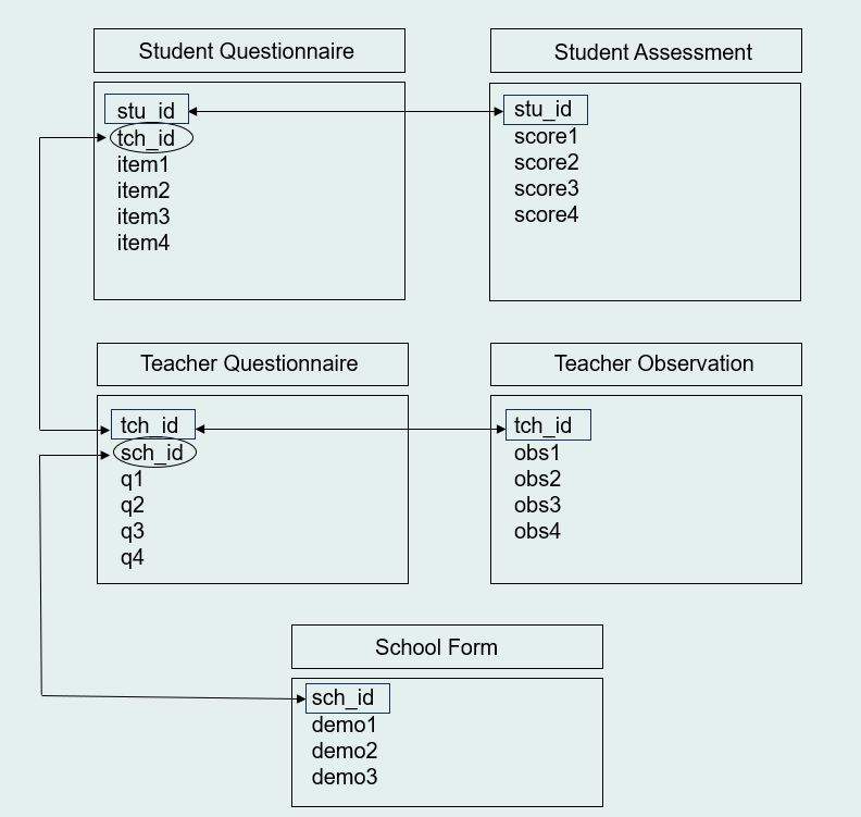
- Each dataset must contain a key.
- There are two types of keys that allow you to link data files—primary and foreign keys. Every dataset should include a primary key that uniquely identifies rows in a dataset. Datasets may also include foreign keys which contain values associated with a primary key in another table. While primary keys cannot include missing or duplicated values, these values are allowed with foreign keys.
- Keys are typically one variable (e.g., a unique study ID), but they may also include more than one variable (e.g., first name + last name), in which case they are called a concatenated key (also called compound or composite key). In the Figure 2, primary keys are denoted by rectangles, and foreign keys are denoted by ovals. Arrows show how data can be linked through both primary and foreign keys.
Left join
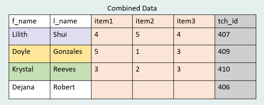
Left joins are probably one of the most common types of joins. While it can be used in many scenarios, this type of join is often helpful to use in the data de-identification process. Let’s say we have a teacher questionnaire dataset + a sample roster dataset.
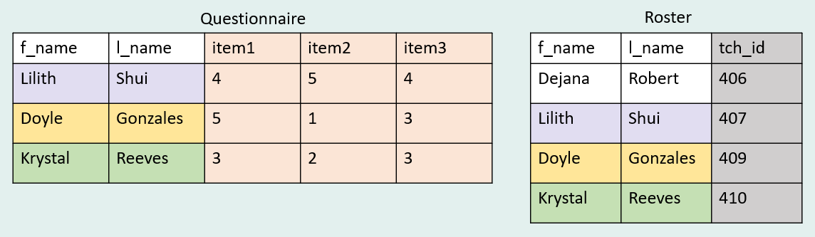
Here we want to add our study ID (tch_id) to our questionnaire. In order to do this, we can join our questionnaire file with a roster file using a combined primary key (f_name and l_name). This works great as long as names are spelled identically across files. 😉
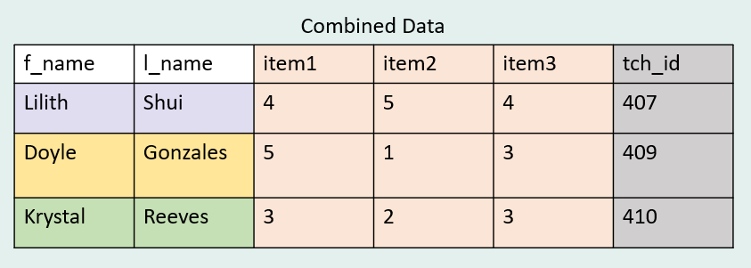
We see that our combined dataset has only three cases which is exactly what we would expect when using a left join. The additional case in our right dataset should not carry over. While we could have used other types of joins, in this scenario we did not want to bring over the information for “Dejana Robert” because she doesn’t exist in our questionnaire data and bringing her in would just create an empty row of data.
Let’s try this join using R. The order of the concatenated key should not matter but I tend to like to merge by last name, then first name. Here I will also fully de-identify the file by removing f_name and l_name after completing the join. I also reordered the variables to put tch_id at the front.
library(dplyr)

tch_svy |>
  left_join(tch_roster, by = c("l_name", "f_name")) |>
  select(tch_id, item1, item2, item3)
NA # A tibble: 3 × 4
NA tch_id item1 item2 item3
NA <dbl> <dbl> <dbl> <dbl>
NA 1 407 4 5 4
NA 2 409 5 1 3
NA 3 410 3 2 3Note While it is typically best practice, and much more convenient, if keys are identically named across files, in programs like R you can still join data even if keys are named differently. See this example where the variable names in the survey are f_name and l_name but in the roster they are first_name and last_name.
library(dplyr)

tch_svy |>
  left_join(tch_roster, by = c("l_name" = "last_name", "f_name" = "first_name")) |>
  select(tch_id, item1, item2, item3)
NA # A tibble: 3 × 4
NA tch_id item1 item2 item3
NA <dbl> <dbl> <dbl> <dbl>
NA 1 407 4 5 4
NA 2 409 5 1 3
NA 3 410 3 2 3Right join
What if, however, we wanted a dataset with our full study sample in it and we did not care whether or not there was missing data for cases? In this case, we could use the same scenario as Figure 2, but instead do a right join (note that we could also just change the order of the datasets and use a left join again). Now when you join your datasets on your compound key, you will end up with four cases in your data.
Let’s try this again using R.
library(dplyr)

tch_svy |>
  right_join(tch_roster, by = c("l_name", "f_name")) |>
  select(tch_id, item1, item2, item3)
NA # A tibble: 4 × 4
NA tch_id item1 item2 item3
NA <dbl> <dbl> <dbl> <dbl>
NA 1 407 4 5 4
NA 2 409 5 1 3
NA 3 410 3 2 3
NA 4 406 NA NA NAFull join
Full joins are very common in research. Imagine a scenario where you are collecting multiple instruments on participants, or you are collecting the same instrument on participants over multiple time points. In those cases, you may have missing data for some participants (i.e., a participant was absent for one of those data collections), but you still want any data that you were able to collect to appear in your combined dataset.
Let’s say you have a student questionnaire + a student assessment. In this case we want all data from both forms to exist in our combined dataset.
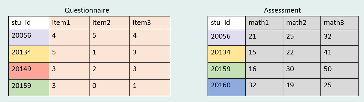
If we performed a full join on these two datasets using stu_id as our key this time, we would expect our final dataset to have 5 cases (or rows). There is one case in each dataset that does not exist in the other.
Let’s see what a full join looks like in R.
library(dplyr)

stu_svy |>
  full_join(stu_assess, by = "stu_id")
NA # A tibble: 5 × 7
NA stu_id item1 item2 item3 math1 math2 math3
NA <dbl> <dbl> <dbl> <dbl> <dbl> <dbl> <dbl>
NA 1 20056 4 5 4 21 25 32
NA 2 20134 5 1 3 15 22 41
NA 3 20149 3 2 3 NA NA NA
NA 4 20159 3 0 1 16 30 50
NA 5 20160 NA NA NA 32 19 25Inner join
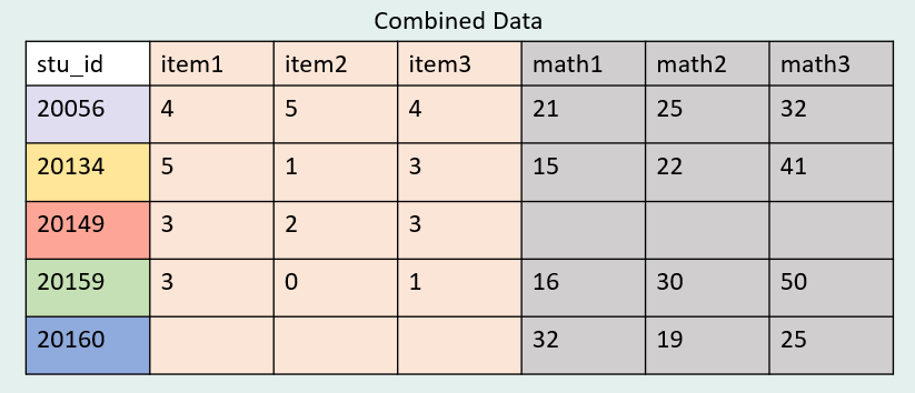
Our last horizontal join type is one that I personally use less often, but there are certainly many scenarios where this will be useful. Let’s take, for instance, the case of a pre and post survey. In this case, we may only want cases in our combined data where a participant has both pre and post data. This is when an inner join can be very useful.
Let’s take a look at our example pre questionnaire + post questionnaire.
Using an inner join we can merge data using our stu_id key again. However, in the case of longitudinal data, our variables are named identically over time which violates one of our horizontal join rules. Therefore, in order to create unique variable names, and to be able to associate each variable with a time point of data collection, we must first concatenate a time period to each repeating variable, before merging data. How time is assigned is completely up to the researcher (read here for more information). In this case, I added the words “pre” and “post” as prefixes, separated by a delimiter for clarity and ease of use.
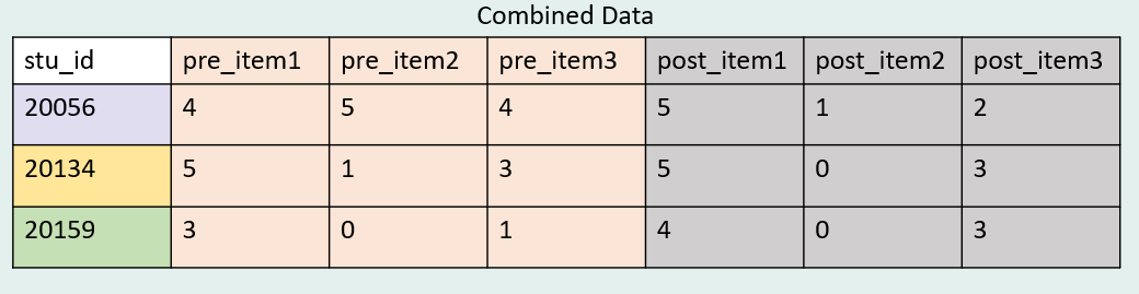
We see that our combined dataset only shows three cases because those are the only cases with both pre and post data available. However, if there had been an empty row for stud_id = 20149 in the post questionnaire data, that case would have been pulled into the combined dataset.
Let’s see what an inner join looks like in R.
library(dplyr)

# First rename variables with pre and post suffix

stu_svy_pre <- stu_svy_pre |>
  rename_with(~ paste0("pre_", .), .cols = -stu_id)

stu_svy_post <- stu_svy_post |>
  rename_with(~ paste0("post_", .), .cols = -stu_id)

# Then join data

stu_svy_pre |>
  inner_join(stu_svy_post, by = "stu_id")
NA # A tibble: 3 × 7
NA stu_id pre_item1 pre_item2 pre_item3 post_item1 post_item2 post_item3
NA <dbl> <dbl> <dbl> <dbl> <dbl> <dbl> <dbl>
NA 1 20056 4 5 4 5 1 2
NA 2 20134 5 1 3 5 0 3
NA 3 20159 3 0 1 4 0 3Note Inner joins are not only for longitudinal data, they can be used for any other other scenarios we discussed. Similarly, longitudinal data can also be joined using any of the other methods we discussed.
Many relationships
Until now we have discussed scenarios that are considered one-to-one merges. In these cases, we only expect one participant in a dataset to be joined to one instance of that same participant in the other dataset.
However, there are scenarios where this will not be the case. Take for instance a case where we are merging information across participant groups (e.g., merging student data with teacher data, or merging teacher data with school data). In these cases, one teacher is often associated with multiple students and one school is often associated with multiple teachers. When we merge data like this, we are working with a one-to-many or a many-to-one merge, depending on which dataset is first or second. In this scenario, we would expect to see repeating data in our combined dataset.
As one example, let’s say we have a student questionnaire + a teacher questionnaire.
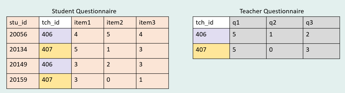
We can combine this data using the tch_id variable which exists in both datasets. However, when we join it will be a one-to-many or a many-to-one join depending on the order of the datasets and which type of join we use.
Let’s say for example, we use a left join, with the student questionnaire dataset on the left and the teacher questionnaire dataset on the right. Here we will be doing a many-to-one join, where each student is associated with multiple teachers—two students will be linked with tch_id = 406 and two students will be linked with tch_id = 407.
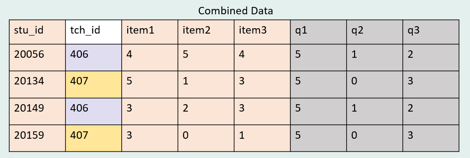
After combining data we see that we have four cases in our data, as we expect from using a left join, but the teacher information we merged in now repeats (twice for each tch_id).
Note The typical rules of a left or right join do not apply when doing a one-to-many join though. Say for example we moved our teacher dataset to the left and performed a left join, this would now be a one-to-many join with one teacher being associated with many students. In this case, the final row number in your combined dataset will not match the count of rows in your original left dataset. Instead it will match the count of the many dataset (i.e., the teacher level dataset will become a student level dataset). So instead of two, the final row final row count would be four.
Let’s perform a many-to-one left join using R, with our student data on the left and our teacher data on the right.
library(dplyr)

stu_svy |>
  left_join(tch_svy, by = "tch_id")
NA # A tibble: 4 × 8
NA stu_id tch_id item1 item2 item3 q1 q2 q3
NA <dbl> <dbl> <dbl> <dbl> <dbl> <dbl> <dbl> <dbl>
NA 1 20056 406 4 5 4 5 1 2
NA 2 20134 407 5 1 3 5 0 3
NA 3 20149 406 3 2 3 5 1 2
NA 4 20159 407 3 0 1 5 0 3Note In dplyr version 1.1.0 or higher, an additional argument was added, relationship. By adding this argument to your join, and specifying the correct type (e.g. one-to-many, many-to-one, one-to-one), you will receive an error if the join violates the constraints of the relationship. Read more here.
Note We did not discuss many-to-many relationships but if you want to see an example of one, you can see an example here.
Vertical joins
Note 2024-01-23 I want to thank the several people who have pointed out that the term “vertical join” is not standard terminology and may be confusing to readers. I acknowledge that stacking data vertically is not technically considered a join (defined as matching dataset rows by a common field/key). So if you are reading this for the first time, please understand that, in this section, I loosely use the term “join” to provide a unifying framework for the different ways you can combine data. However, when you are doing “vertical joins”, more appropriate terms to use would include append, stack, or union data.
Similar to horizontal joins, there are many use cases for joining data vertically, also called appending data (or union in SQL). Some examples include:
- Combining similar data across cohorts
- Combining similar data collected from different sites or links
- Combining similar data collected across time
However, there are some fundamental differences between horizontal and vertical joins. 1. Rather than joining data on keys, columns are matched by variable names. 2. In this case you do not want unique variable names. Here, it is imperative that variables are named and formatted identically across datasets.
Note Not all functions/statements match on column names. Some match on column order. Make sure to understand the program/function you are working with before appending data. Similarly, not all functions will require that your variable types (e.g., numeric, character) be identical across datasets. However, it is still good practice, no matter which function you use, to keep types consistent across datasets that you plan to append.
Let’s take an example where we have a questionnaire collected across two cohorts of teachers. We can append these data, creating a longer dataset. The inclusion of the cohort variable allows users to know which data is associated with which cohort in the combined data.
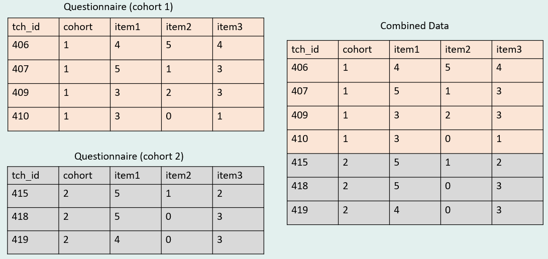
Let’s see what this type of join would look like in R.
First, let’s check that the variable names and types are identical across datasets.
library(janitor)

compare_df_cols(svy_c1, svy_c2)
NA column_name svy_c1 svy_c2
NA 1 cohort numeric numeric
NA 2 item1 numeric numeric
NA 3 item2 numeric numeric
NA 4 item3 numeric numeric
NA 5 tch_id numeric numericOur column names and types are identical so we are good to go.
library(dplyr)

bind_rows(svy_c1, svy_c2)
NA # A tibble: 7 × 5
NA tch_id cohort item1 item2 item3
NA <dbl> <dbl> <dbl> <dbl> <dbl>
NA 1 406 1 4 5 4
NA 2 407 1 5 1 3
NA 3 406 1 3 2 3
NA 4 407 1 3 0 1
NA 5 415 2 5 1 2
NA 6 418 2 5 0 3
NA 7 419 2 4 0 3Note When using bind_rows(), if any variables are not identically named and formatted across datasets, you will get an error.
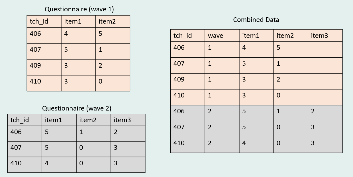
You can also append longitudinal data. For example, if your repeated measures analysis requires data to be in long format, rather than wide (as seen with horizontal joins), longitudinal data can be vertically joined. In this case, rather than concatenating a time component to your time varying variables, a time variable is added to the data to delineate which rows belong to which time period. How a time component is assigned is completely up to you. Here I chose to add a variable named wave and assign numeric values to my time points (read here for more information).
Note Even if one dataset contains variables that do not exist in the other (e.g., a variable was added to the questionnaire at a later time), appending will still work when using bind_rows(). This may not be true for other binding functions/statements.
Let’s see this done using R.
library(dplyr)

# First add a wave variable

svy_w1 <- svy_w1 |>
  mutate(wave = 1)

svy_w2 <- svy_w2 |>
  mutate(wave = 2)

# Then append data

bind_rows(svy_w1, svy_w2) |>
  relocate(wave, .after = tch_id)
NA # A tibble: 7 × 5
NA tch_id wave item1 item2 item3
NA <dbl> <dbl> <dbl> <dbl> <dbl>
NA 1 406 1 4 5 NA
NA 2 407 1 5 1 NA
NA 3 409 1 3 2 NA
NA 4 410 1 3 0 NA
NA 5 406 2 5 1 2
NA 6 407 2 5 0 3
NA 7 410 2 4 0 3Note Notice now that tch_id no longer uniquely identifies rows in our combined dataset. When appending longitudinal data, we now have a concatenated primary key that uniquely identifies rows (tch_id + wave)
Combining joins
In large research studies, it is common to combine horizontal and vertical joins. Take for instance a study that collects two waves of a teacher questionnaire, for two cohorts.
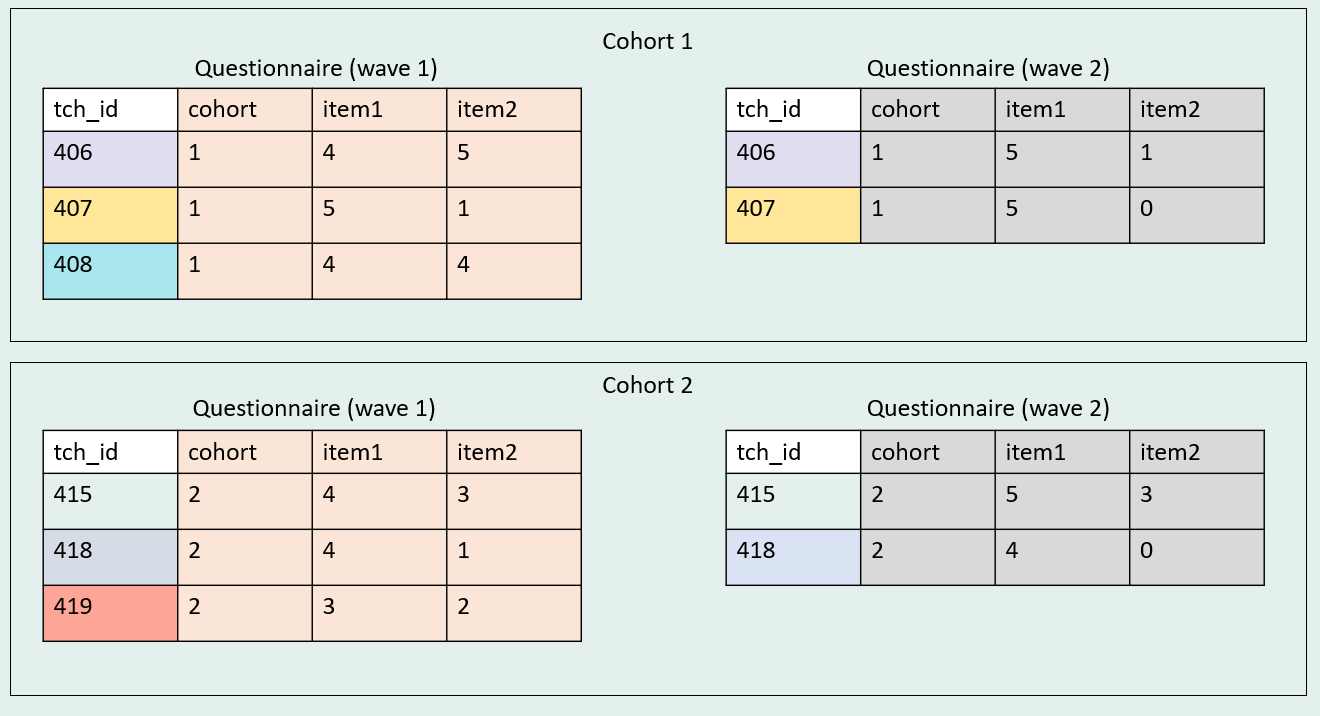
This data can be combined in many ways depending on your needs. One way we could combine this data might be - First, horizontally join within cohort. Here I am choosing to do a full join. - Then, append the cohorts.
Note Since cohort appears in both datasets and we are joining horizontally, we will need to make a decision on which cohort variable to keep in our full join. We do not want to keep both, not only because this will cause confusion, but also because they are identically named, violating one of our rules of horizontal joins. In both cases, I choose to drop the cohort variable from the right side dataset because the left side dataset has the most complete information. This will not always be the case. In some cases, you may need to use the right side or combine information across both variables into one complete variable.
1. Let’s first join cohort 1.
library(dplyr)

# First rename variables with wave 1 (w1) and wave 2 (w2) suffix
# Also, drop cohort from the wave 2 dataset

tch_svy_w1_c1 <- tch_svy_w1_c1 |>
  rename_with(~ paste0("w1_", .), .cols = -c(tch_id, cohort))

tch_svy_w2_c1 <- tch_svy_w2_c1 |>
  rename_with(~ paste0("w2_", .), .cols = -c(tch_id, cohort)) |>
  select(-cohort)

# Then horizontally join across waves

tch_svy_w1w2_c1 <- tch_svy_w1_c1 |>
  full_join(tch_svy_w2_c1, by = "tch_id")


tch_svy_w1w2_c1
NA # A tibble: 3 × 6
NA tch_id cohort w1_item1 w1_item2 w2_item1 w2_item2
NA <dbl> <dbl> <dbl> <dbl> <dbl> <dbl>
NA 1 406 1 4 5 5 1
NA 2 407 1 5 1 5 0
NA 3 408 1 4 4 NA NA2. Next let’s join cohort 2.
# First rename variables with wave 1 (w1) and wave 2 (w2) suffix
# Also, drop cohort from the wave 2 dataset

tch_svy_w1_c2 <- tch_svy_w1_c2 |>
  rename_with(~ paste0("w1_", .), .cols = -c(tch_id, cohort))

tch_svy_w2_c2 <- tch_svy_w2_c2 |>
  rename_with(~ paste0("w2_", .), .cols = -c(tch_id, cohort)) |>
  select(-cohort)

# Then horizontally join across waves

tch_svy_w1w2_c2 <- tch_svy_w1_c2 |>
  full_join(tch_svy_w2_c2, by = "tch_id")


tch_svy_w1w2_c2
NA # A tibble: 3 × 6
NA tch_id cohort w1_item1 w1_item2 w2_item1 w2_item2
NA <dbl> <dbl> <dbl> <dbl> <dbl> <dbl>
NA 1 415 2 4 3 5 3
NA 2 418 2 4 1 4 0
NA 3 419 2 3 2 NA NA3. Now we can append the cohorts.
bind_rows(tch_svy_w1w2_c1, tch_svy_w1w2_c2)NA # A tibble: 6 × 6
NA tch_id cohort w1_item1 w1_item2 w2_item1 w2_item2
NA <dbl> <dbl> <dbl> <dbl> <dbl> <dbl>
NA 1 406 1 4 5 5 1
NA 2 407 1 5 1 5 0
NA 3 408 1 4 4 NA NA
NA 4 415 2 4 3 5 3
NA 5 418 2 4 1 4 0
NA 6 419 2 3 2 NA NANote We don’t have to combine data this way. We could change the order of how we join data (i.e., append cohorts first, then horizontally join waves), or we could change the structure of the data completely (e.g., append waves in long format, as well as append cohorts, creating a very long dataset).
Let’s look at one more scenario where we are combining joins. In this case we have a teacher questionnaire collected across two waves, and we have school-level demographic data, also collected across two waves.
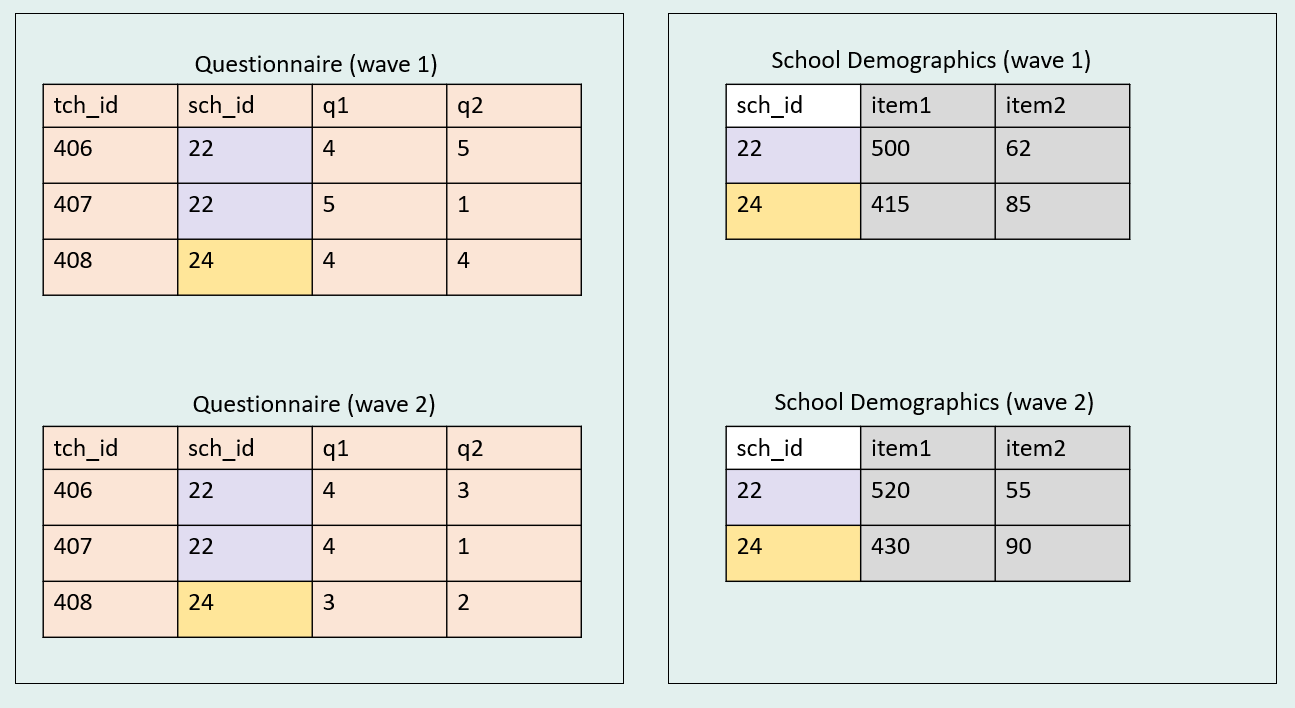
Again, we could combine this data in multiple ways, but here we are going to - First, append the two waves of data into long format. - Then, horizontally join the school data using a left join.
1. Append within teacher data.
# First add a wave variable

tch_svy_w1 <- tch_svy_w1 |>
  mutate(wave = 1)

tch_svy_w2 <- tch_svy_w2 |>
  mutate(wave = 2)

# Then append

tch_svy <- bind_rows(tch_svy_w1, tch_svy_w2) |>
  relocate(wave, .after = tch_id)

tch_svy
NA # A tibble: 6 × 5
NA tch_id wave sch_id q1 q2
NA <dbl> <dbl> <dbl> <dbl> <dbl>
NA 1 406 1 22 4 5
NA 2 407 1 22 5 1
NA 3 408 1 24 4 4
NA 4 406 2 22 4 3
NA 5 407 2 22 4 1
NA 6 408 2 24 3 22. Append within school data.
# First add a wave variable

sch_w1 <- sch_w1 |>
  mutate(wave = 1)

sch_w2 <- sch_w2 |>
  mutate(wave = 2)

# Then append

sch_svy <- bind_rows(sch_w1, sch_w2) |>
  relocate(wave, .after = sch_id)

sch_svy
NA # A tibble: 4 × 4
NA sch_id wave item1 item2
NA <dbl> <dbl> <dbl> <dbl>
NA 1 22 1 500 62
NA 2 24 1 415 85
NA 3 22 2 520 55
NA 4 24 2 430 903. Then left join teacher data with school data.
Note Notice that because we have longitudinal data appended in long format, I have to use a concatenated primary key to join our data.
tch_svy |>
  left_join(sch_svy, by = c("sch_id", "wave"))
NA # A tibble: 6 × 7
NA tch_id wave sch_id q1 q2 item1 item2
NA <dbl> <dbl> <dbl> <dbl> <dbl> <dbl> <dbl>
NA 1 406 1 22 4 5 500 62
NA 2 407 1 22 5 1 500 62
NA 3 408 1 24 4 4 415 85
NA 4 406 2 22 4 3 520 55
NA 5 407 2 22 4 1 520 55
NA 6 408 2 24 3 2 430 90Checks
No matter what type of join you use, make sure to always review your data after combining it to check that you have the expected number of cases. It’s very easy to make a mistake in your joining process and end up with duplicate rows you didn’t expect or accidentally dropping rows you meant to keep. So always check your row count after combining data to ensure that no mistakes were made in the process.
Additional resources
This blog post is just a primer to get you started thinking about joins. There are many more types of joins, as well as many more combinations of joins that can be used! In the end, it all depends on what is useful for your project and your purposes (read here for more information). Also, just because you can join data, doesn’t mean you need to rush into it. The flat file format datasets often used in research (e.g., CSV files) can be easily stored separately until it becomes necessary for you to join them. I usually think this is the best method because it allows you to more easily update individual files as needed, and it prevents you from potentially joining in a way that is ultimately not necessary or not aligned with what is needed (more information can be found here).
For further learning, check out these additional very helpful resources!
Post updated 2024-11-16
Citation
BibTeX citation:
@online{lewis2024,
  author = {Lewis, Crystal},
  title = {Let’s Talk about Joins},
  date = {2024-01-10},
  url = {https://cghlewis.com/blog/joins/},
  langid = {en}
}
For attribution, please cite this work as:
Lewis, Crystal. 2024. “Let’s Talk about Joins.” January 10.
https://cghlewis.com/blog/joins/.